Measure the gap
Calculate the angle between the current orbit and the target orbit.
My dissertation asks a practical question: how much debris could one spacecraft remove from Sun synchronous orbit within a fixed propellant budget? I built the study around 637 catalogued objects between 550 and 750 km.
Reaching this region is not the main difficulty. Instead, the main challenge is moving from one orbital plane to another. Even a small change between two near polar orbits can use most of the available propellant.
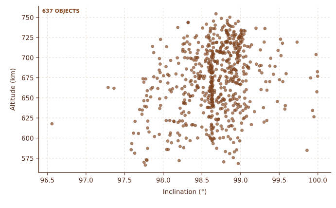
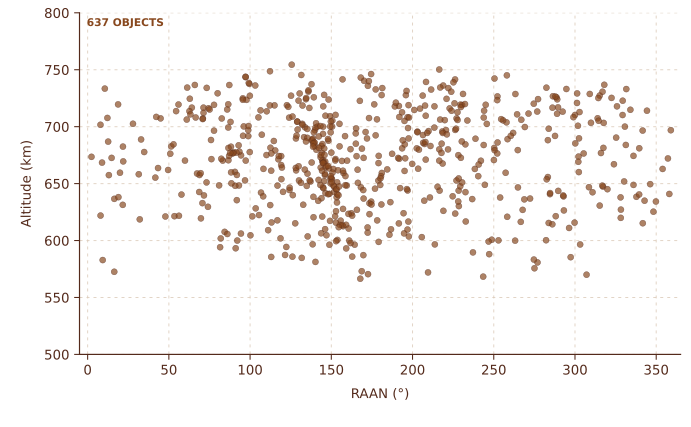
Earth is slightly wider at the equator than at the poles. As a result, its uneven gravity slowly rotates an orbit's plane. This effect is called \(J_2\) precession, and its rate changes with altitude and inclination.
I used this drift to reduce the burn needed for the plane change. The spacecraft first enters a temporary orbit. It then waits. Once its plane reaches the target's plane, it returns to the parking altitude.
Calculate the angle between the current orbit and the target orbit.
Use two small burns to enter the selected drift orbit.
Let the difference in \(J_2\) precession close the RAAN gap.
Move back to the parking altitude once the planes align.
I wrote a Python planner to test this across a full mission. Before each transfer, it considers every object that has not yet been visited. For each candidate it tests 20 drift altitudes and 30 drift times. It then calculates the inclination needed to meet the target plane. Orbits outside the limits of the study are rejected.
Each feasible transfer has two costs: propellant and time. Waiting longer can make a transfer cheaper, but it can also leave the spacecraft drifting for years. I therefore gave the planner a setting that controls how strongly it penalises waiting. A low penalty favours cheaper burns, whereas a higher one keeps the mission shorter.
After scoring the transfers, the planner selects the lowest cost target. It then updates the RAAN of the spacecraft and every object still in the catalogue before repeating the search. The mission ends when no further transfer fits within the \(500\,\mathrm{m\,s^{-1}}\) budget. Because one decision changes the geometry of the next, the route can change when the time penalty changes.
A single transfer shows how much the drift can matter. With a \(3^{\circ}\) RAAN gap and a \(0.2^{\circ}\) difference in inclination, a direct round trip costs \(781.0\,\mathrm{m\,s^{-1}}\) in the model. By comparison, allowing \(259.3\) days for natural \(J_2\) drift reduces the cost to \(4.20\,\mathrm{m\,s^{-1}}\). This uses \(99.5\%\) less propellant.
When the planner minimises only propellant, it removes 13 objects using \(363.0\,\mathrm{m\,s^{-1}}\) and takes 8.34 years. By contrast, the run I selected gives more weight to time. It removes 19 objects in 1.65 years using \(440.7\,\mathrm{m\,s^{-1}}\). This remains below the \(476.2\,\mathrm{m\,s^{-1}}\) reserve limit.
This is a planning study, not a flight design. Between transfers, the model propagates only \(\Omega\). Consequently, it does not include in plane phasing or short period motion. The search also chooses one transfer at a time, so it cannot guarantee the best route through the full catalogue. Rendezvous and capture would need a separate study.